A Text book for OMNeT++ (Learning OMNeT++)

This post is for the nsnam.com readers particularly those who want to learn OMNeT++. As you aware, ns2 and OMNeT++ are two software that are freely distributed and available to academics for almost free of cost.

However, when dealing with the documentation, both suffers a set back. NS has a documentation and still researchers across the world have their own way of learning. And OMNeT++ has a proper documentation, that is very huge and takes times to understand.
Packt Publishing has published a book in OMNeT++ authored by Thomas Chamberlain
You may refer the following website for http://www.packtpub.com/
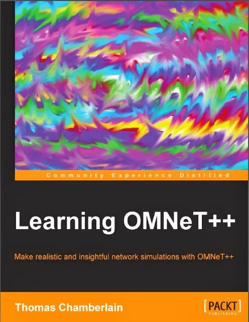
Omnet++
OMNeT++
You can also learn: http://www.nsnam.com/2013/12/installation-of-omnet-in-linux-mint-16.html
This book is organized in the following chapters.

  • Getting started with OMNeT++
  • Installing OMNeT++
  • OMNeT++ Simulations 
  • Creating and Running simulation
  • Learning from your simulation
There are just 5 chapters that are just enough for a beginner to get a grip in understanding  OMNeT++. Also the book contains just 102 pages and one can learn this book within a day or two.


T S Pradeep Kumar

Comments

Popular posts from this blog

Installing ns3 in Ubuntu 22.04 | Complete Instructions

In this post, we are going to see how to install ns-3.36.1 in Ubuntu 22.04. You can follow the video for complete details Tools used in this simulation: NS3 version ns-3.36.1  OS Used: Ubuntu 22.04 LTS Installation of NS3 (ns-3.36.1) There are some changes in the ns3 installation procedure and the dependencies. So open a terminal and issue the following commands Step 1:  Prerequisites $ sudo apt update In the following packages, all the required dependencies are taken care and you can install all these packages for the complete use of ns3. $ sudo apt install g++ python3 python3-dev pkg-config sqlite3 cmake python3-setuptools git qtbase5-dev qtchooser qt5-qmake qtbase5-dev-tools gir1.2-goocanvas-2.0 python3-gi python3-gi-cairo python3-pygraphviz gir1.2-gtk-3.0 ipython3 openmpi-bin openmpi-common openmpi-doc libopenmpi-dev autoconf cvs bzr unrar gsl-bin libgsl-dev libgslcblas0 wireshark tcpdump sqlite sqlite3 libsqlite3-dev  libxml2 libxml2-dev libc6-dev libc6-dev-i386 libclang-dev llvm-

Installation of NS2 (ns-2.35) in Ubuntu 20.04

Installation of NS2 (ns-2.35) in Ubuntu 20.04 LTS Step 1: Install the basic libraries like      $] sudo apt install build-essential autoconf automake libxmu-dev Step 2: install gcc-4.8 and g++-4.8 open the file using sudo mode $] sudo nano /etc/apt/sources.list Include the following line deb http://in.archive.ubuntu.com/ubuntu bionic main universe $] sudo apt update $] sudo apt install gcc-4.8 g++-4.8 Step 3:  Unzip the ns2 packages to home folder $] tar zxvf ns-allinone-2.35.tar.gz $] cd ns-allinone-2.35/ns-2.35 Modify the following make files. ~ns-2.35/Makefile.in Change @CC@ to gcc-4.8 change @CXX@ to g++-4.8 ~nam-1.15/Makefile.in ~xgraph-12.2/Makefile.in ~otcl-1.14/Makefile.in Change in all places  @CC@ to gcc-4.8 @CPP@ or @CXX@ to g++-4.8 open the file: ~ns-2.35/linkstate/ls.h Change at the Line no 137  void eraseAll() { erase(baseMap::begin(), baseMap::end()); } to This void eraseAll() { this->erase(baseMap::begin(), baseMap::end()); } All changes made Step 4: Open a new termi

Square and Sinusoidal Waveform in 8051 Microcontroller

Waveforms in 8051 Microcontroller Square Wave To create a square wave generation using Delay. let us say we want to construct a 1khz square waveform the processor instruction cycle of 8051 is 1.085microseconds so for 1khz (1milli seconds =1/1khz), is 1ms/1.085microseconds = 921.6 (this value is set to the for loop) #include <reg51.h> void delay() { int i=0; for(i=0;i<922;i++) } void main() { P0=0xff; delay(); P0=0x00; delay(); } Sine Wave generation Since sine wave is plotted in a digital device the number of samples determines the smoothness, hence in this case, more the samples, smoother is the waveform. so a lookup table is been created to get the samples. in the following examples, there are totally 36 samples are taken, starting from 0 degrees to 360 degrees with a step of 10 degrees Degrees A = 5 (1+Sin theta) Where 5 is the full scale voltage DAC = 25.6 * A 0 5 128 30 7.5 192 60 9.3 239 90 10 256 etc…like this we need to calculate for 13 samples  with a ste