
Wireless Networks
In this post:
Introduction to Wireless Networks
Tcl scripts for various wireless networks
Unlike Wired networks, wireless networks are a little tricky in dealing with the network properties. Since wireless nodes have radio, physical layer, Mac (Medium Access Control), Antenna, etc. Every parameter of those should be addressed when configuring wireless networks.
NS provides a way to handle these properties through a construct called node-config. The node configuration in ns2 is a special task in which the number of nodes can be configured for a set of parameters. The following table tells about the node configuration parameters as defined in the ~ns-2.35/tcl/ns-lib.tcl
The readers are requested to refer the ns-lib.tcl file for more information.
6.1 Wireless Node Configuration
The following table shows the complete node configuration that ns supports or provides. The wireless nodes may be configured with all the parameters given here or whatever is needed can be used to configure.
An Example
$ns node-config -addressType hierarchical \
-adhocRouting AODV \
-llType LL \
-macType Mac/802_11 \
-ifqType Queue/DropTail/PriQueue \
-antType Antenna/OmniAntenna \
-propType Propagation/TwoRayGround \
-phyType Phy/WirelessPhy \
-topologyInstance $topo \
-energyModel “EnergyModel” \
-initialEnergy 3.0 \
-txPower 0.3 \
-rxPower 0.1 \
-sleepPower 0.05 \
-idlePower 0.08 \
-channel Channel/WirelessChannel \
-agentTrace ON \
-routerTrace OFF \
-movementTrace ON \
-macTrace OFF
6. 2 A Simple Wireless Configuration
For every node creation, the above node-config has to be set in the wireless networks. Now we will see a simple example related to wireless networks.
The Listing 6.1 shows the wireless network with two nodes that involves in a exchange of information. This network generates two files a network animator file (wrls1.nam) and a trace file (wrls1.tr)
The output of the tracefile is, here it shows the first few lines of the wrls1.tr
s 0.029290548 _1_ RTR --- 0 message 32 [0 0 0 0] ------- [1:255 -1:255 32 0]
s 0.029365548 _1_ MAC --- 0 message 90 [0 ffffffff 1 800] ------- [1:255 -1:255 32 0]
r 0.030085562 _0_ MAC --- 0 message 32 [0 ffffffff 1 800] ------- [1:255 -1:255 32 0]
r 0.030110562 _0_ RTR --- 0 message 32 [0 ffffffff 1 800] ------- [1:255 -1:255 32 0]
s 1.119926192 _0_ RTR --- 1 message 32 [0 0 0 0] ------- [0:255 -1:255 32 0]
s 1.120361192 _0_ MAC --- 1 message 90 [0 ffffffff 0 800] ------- [0:255 -1:255 32 0]
r 1.121081207 _1_ MAC --- 1 message 32 [0 ffffffff 0 800] ------- [0:255 -1:255 32 0]
r 1.121106207 _1_ RTR --- 1 message 32 [0 ffffffff 0 800] ------- [0:255 -1:255 32 0]
Here is the analysis of the above trace file
ACTION: [s|r|D]: s -- sent, r -- received, D – dropped
WHEN: the time when the action happened
WHERE: the node where the action happened
LAYER:
AGT -- application,
RTR -- routing,
LL -- link layer (ARP is done here)
IFQ -- outgoing p’acket queue (between link and mac layer)
MAC -- mac,
PHY – physical
flags:
SEQNO: the sequence number of the packet
TYPE: the packet type cbr -- CBR data stream packet
DSR -- DSR routing packet (control packet generated by routing)
RTS -- RTS packet generated by MAC 802.11
ARP -- link layer ARP packet
SIZE: the size of packet at current layer, when packet goes down, size increases, goes up size decreases[a b c d]: a -- the packet duration in mac layer header b -- the mac address of destination c -- the mac address of source d -- the mac type of the packet body
flags:
[......]: [ source node ip : port_number destination node ip (-1 means broadcast) : port_number ip header ttl ip of next hop (0 means node 0 or broadcast) ]
So we can interpret the below trace
r 0.010176954 _9_ RTR --- 1 gpsr 29 [0 ffffffff 8 800] ------- [8:255 -1:255 32 0]
in the same way, as The routing agent on node 9 received a GPSR broadcast (mac address 0xff, and ip address is -1, either of them means broadcast) routing packet whose ID is 1 and size is 19 bytes, at time 0.010176954 second, from node 8 (both mac and ip addresses are 8), port 255 (routing agent)
The output of the network animation file is
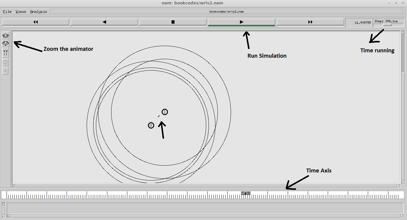
Fig 6.1 – Network Animation Window
This example though it performs a little work, but the results it gives are tremendous. There are so many parameters that change during the execution of the network. Some of the performance characteristics are listed:
Throughput of Generating packets or sending packets
End to End delay between the nodes
Packet Delivery ratio.
Packet loss and packet drop calculation
Jitter
Energy used by the nodes
And so many other parameters.
These parameters are calculated based on the contents of the trace file. There are so many softwares available to process these trace files. Xgraph is a utility that comes with ns-allinone package and is very useful to predict the performance metrics. There are other third party software that can be used to process these trace files,
Tracegraph
Tracegraph is not actively maintained and it is using matlab runtime libraries.
It does not process the energy values in the trace file
Very easy to handle, just open the file using a GUI windows and rest taken care by the software.
Its free and open source. This software can be downloaded at [5].
More information about Tracegraph and GnuPlot is available at Appendix D
GnuPlot
This is also free and easy to handle
Need to specify the axis manually and results are great looking.
Matlab
Its runtime libraries are responsible for processing the data.
It’s a proprietary software
AWK programming language
Its one of the powerful programming language that can process the data column wise.
Its open source and free. Refer Appendix B for more information
Analysis using Tracegraph, Listing 6.1 has two nodes that involves a TCP traffic flow and the nodes were moving. In this case, at the end of the simulation, both the nodes were away from each other and a packet drop and packet loss occurs. These results can be predicted using tracegraph as indicated below.
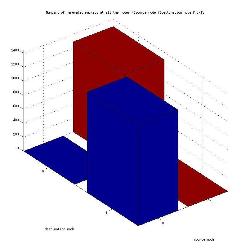
Fig 6.2 - A 3d Graph that shows the generation of packets at all the nodes
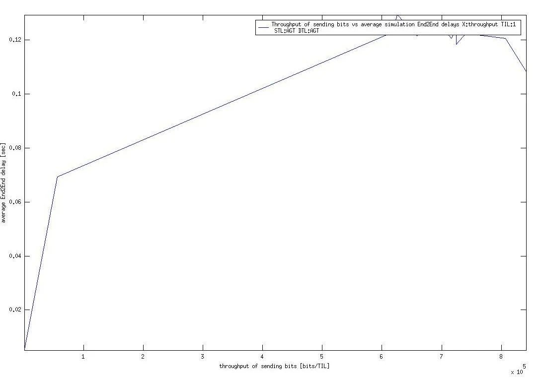
Fig 6.3 – Average End to End delay for Sending bits
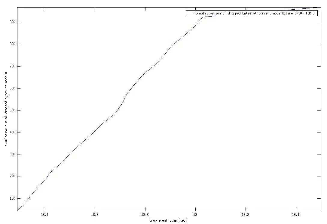
Fig 6.4 – Cumulative sum of dropped bytes of RTS packets at all nodes
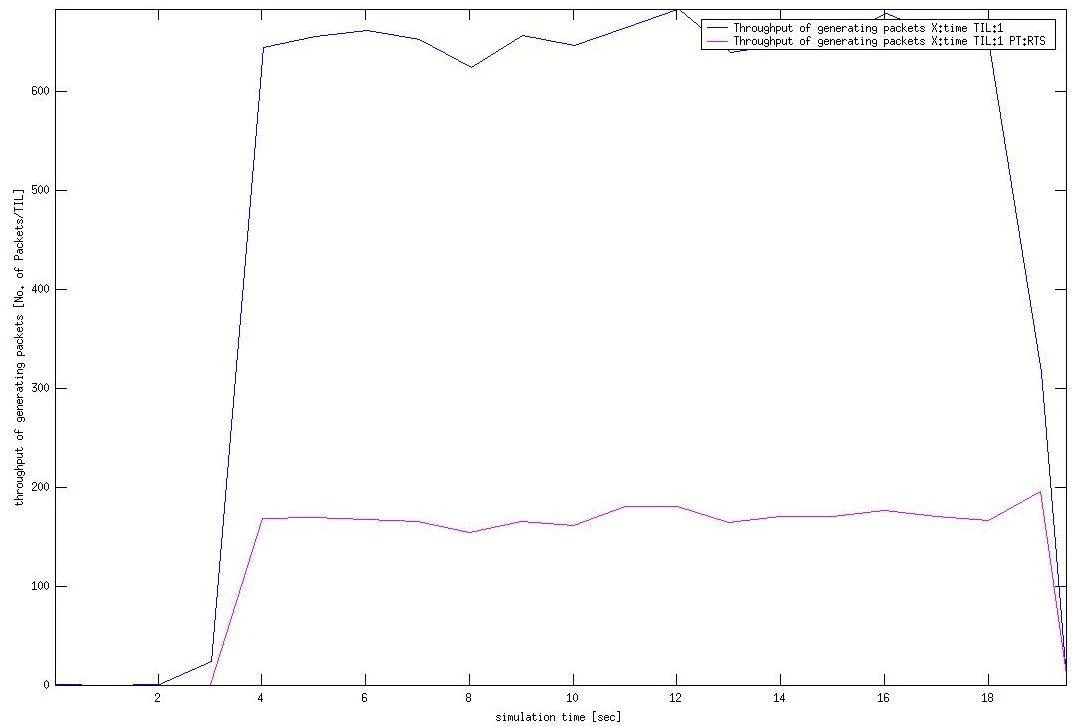
Fig 5.5 – Throughput of all generated packets at all nodes.
The above graphs, plots the various performance characteristics of the given wireless network and each graph tells some information about the network. For example, in the above graph, there are two waveforms, one refers the throughput of generating packets at all nodes and the smaller one refers the throughput of generating packets of RTS at all nodes. From the fig5.5, it was assumed that the RTS packets are limited in generation compared with the other packets in the network.
Also the tracegraph software will present the text based information about the network. The following Fig 5.6 and Fig 5.7 shows that
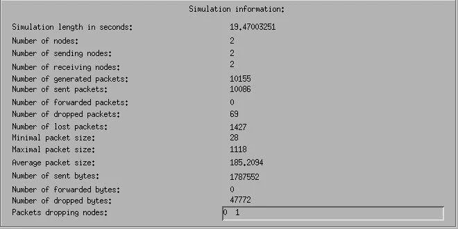
Fig 6.6 – Simulation Information
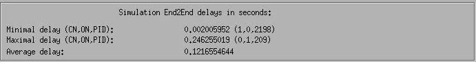
Fig 6.7 – End to End delay
The simulation information shows the number of dropped packets is 69 and lost packets are 1427 and both the nodes (0 and 1) are dropping the packets.
6.3 Energy Model in Wireless networks
Real wireless nodes are equipped with battery that will last long only when the batteries are charged. In a simulator environment, implementing a battery model is always challenging as the battery has a non linear characteristics. However, ns implements a energy model for wireless nodes that uses functions based on the energy usage of the nodes during transmitting, receiving, sleeping and even when the nodes are idle. In Listing 6.1, the nodes are not enabled with energy model, hence the nodes uses infinite amount of energy which in practice is extinct. Listing 6.2 implements energy model for the nodes as listed below:
Energy unit is given in Joules and Power consumption is calculated based on usage in Watts
As we know the energy and power relation is
Power X Time = Energy,
As per the above equation, even when the node is sleeping or idle, power is consumed as we use our real Smart Phones or Mobile phones (that consumes power or the antenna is always on to receive the signal)
In the Listing 6.2, the following codes are added for including energy model into the nodes
-energyModel "EnergyModel" \
-initialEnergy 3.2 \
-txPower 0.3 \
-rxPower 0.1 \
-sleepPower 0.05 \
-idlePower 0.1 \
These codes includes the energy consumption while
Transmitting
Receiving
Sleeping
Even when the node is idle
Transition energy also is one of the factor
The output trace file includes extra column for energy usage too.as shown below
s 0.032821055 _1_ RTR --- 0 message 32 [0 0 0 0] [energy 3.200000 ei 0.000 es 0.000 et 0.000 er 0.000] ------- [1:255 -1:255 32 0]
The bold letters in the above line indicates the energy level trace.
energy – initial energy value which is given as 3.2 Joules
ei – idle energy
es – sleep energy
et – transmission energy
er – reception energy
Fig 5.8 shows the picture of energy level Nodes. The figure shows the nodes are in Green color and when the node’s energy comes to a threshold value, it changes to yellow and if the energy completely drained then the nodes die indicated by changing the color to red.
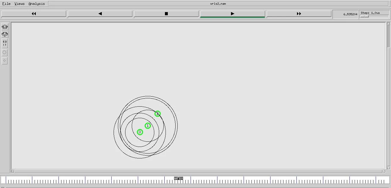
Fig 5.8 – Wireless network with energy Model
6.4 – Performance characteristics in Wireless Adhoc networks
The Listing 6.3 uses
8 wireless nodes with adjusted mac parameters
UDP Agent for Source agent
LossMonitor agent to trace the received bytes
Each agent has a priority value from ( 0 to 3). There are four flows
The characteristics that were plotted are
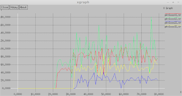
Packet loss
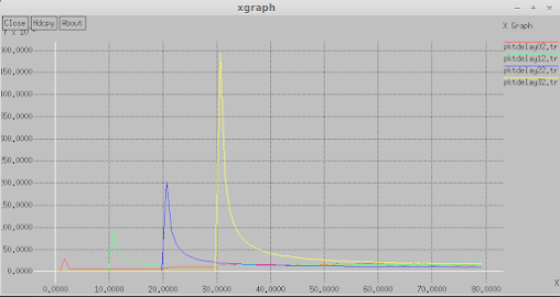
Packet Delay
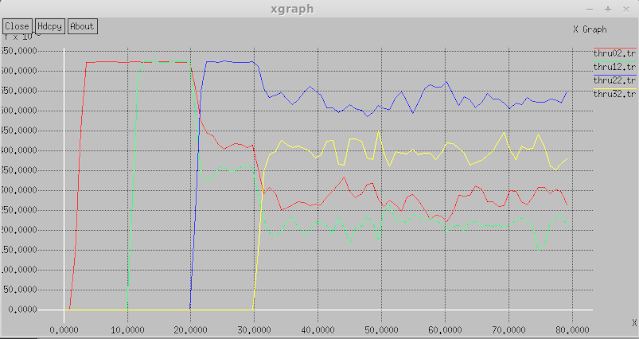
Throughput
The Network animation looks likes the following (8 nodes with packet exchange)
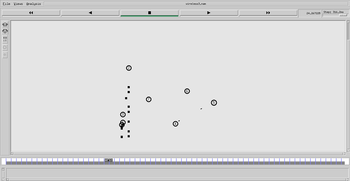
And the characteristics are shown below
Packet Delay for various traffic flow
Packet Loss for various traffic flows
Throughput for various traffic flows.
6.5 Message Sending in Wireless Networks
6.7 Conclusion:
This chapter deals with the basics of wireless adhoc networks and their simulation in NS2. This chapter shows the wireless networks with two nodes, energy model enablement and message sending between the nodes. For most of the 802.11 mac protocols, the same set of node configuration, GOD object setting, Agent creation, etc, will be common. Using this chapter, one can able to design most of the wireless ad hoc networks in NS2.
Comments
Post a Comment